Diffusion. What is it?
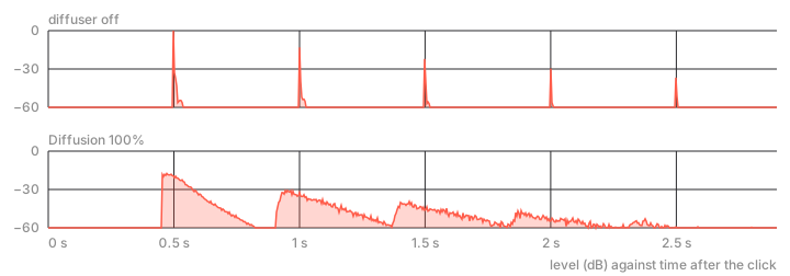
What's a diffuser? Basically smearing a bunch of tap repeats across time!
Note: This one leans on the EQ post a lot, so if \(z^{-1}\) and the unit circle are fuzzy, start there. There's more maths this time, but most of it is one trick.
What a diffuser does
You ever try singing in the shower? Clapping in a stairwell? Yodeling over a canyon? The sound waves you produce bounce off every surface, then off every other surface, off you, off invisible particles in the air (in the case of singing in the shower, water in the air), so on, so forth. That's diffusion! Cathedrals aren't that big for no reason!
You can think of a delay repeat as a sort of degraded mirror image. The physics of the degradation is pretty simple; repeats lose energy as they come into into contact with air resistance, particles in the air, materials with different absorption coefficients, etc etc. This degradation is important because it is through this interaction which a plugin will gain its "signature sound". Every material an impulse bounces off of imparts a characteristic quality, or a form of coloration onto the wave, which we can model and control. Chronos's diffuser sits inside the feedback loop, so every repeat gets smeared, then smeared again on the next lap. After a few laps the repeats melt into a wash.
The thing is, it has to smear time without touching the tone. Say the diffuser boosted 2 kHz by 1 dB. It's in the loop, so ten repeats later that's 10 dB; you end up with a less than ideal result (it'd sound like a whistle in this case). A filter with a dead flat frequency response that still scrambles time is necessary here. In Electrical Engineering, this is what is called an Allpass Filter.
Make a note of these symbols:
| \(f_s\) | sample rate, 48,000 here |
| \(M\) | a delay length, in samples |
| \(n\) | a counter. In \(x[n]\), it counts samples. In the echo series \(w^n\), it counts laps through the pipe |
| \(nM\) | \(n\) times \(M\): the total delay after \(n\) laps. With \(M = 113\), the third echo arrives at \(3 \times 113 = 339\) samples |
| \(z^{-M}\) | "M samples ago": the EQ post's \(z^{-1}\), M times over |
| \(g\) | the allpass coefficient, what the Diffusion knob turns. Not the EQ post's \(g\), sorry, everyone calls this one g too |
| \(\theta\) | the angle round the unit circle, \(\theta = 2\pi f/f_s\) |
| \(h[n]\) | the impulse response: what comes out when you put in one click |
| \(\bar{w}\) | \(w\)'s mirror image below the x-axis (the complex conjugate) |
Running numbers: \(f_s = 48{,}000\), \(M = 113\) samples (Chronos's first section, about 2.35 ms) and \(g = 0.78\) (Diffusion all the way up).
A delay with feedback is a comb
Lets start with something simple, like a delay with feedback: turn the output down by \(g\) and add it back in, \(M\) samples later.
The feedback in an EQ is instant (that was the whole zero-delay thing from the EQ post). Here it takes \(M\) samples to come back round.
Input some arbitrary source, where the first tap = 1, then \(g\) = 0.78, then \(g^2\) = 0.61 and so on, \(M\) samples apart. You can immediately see how important the \(M\) variable is. At 500 ms, this is proper delay. At something like \(M = 113\) or 2.35ms, you end up with pitch mod: \(48000/113 \approx 425\) Hz. That metallic ring is a comb filter.
Mathematically this is just filter design. Swap \(y[n-M]\) for \(z^{-M}Y\) and solve:
An audible tone = a counter-clockwise "walk" around the unit circle.
\(z = e^{j\theta}\), so \(z^{-M} = e^{-jM\theta} = \cos M\theta - j\sin M\theta\).
Split the denominator into its real and imaginary parts:
Length squared is \(\cos^2 + \sin^2 = 1\):
The cosine works here by making the response rise and fall as the frequency goes up, like a sort of wobble. The peaks happen where \(\cos M\theta = 1\), spaced \(f_s/M\) hertz apart (every 425 Hz here). The "dips" sit halfway between them. To see how big that wobble is, divide the peak by the dip:
With \(g = 0.78\) that's \(1.78/0.22 \approx 8.1\), about 18 dB of ripple. On every lap? Not a coloration we really want. Undesirable result!
What do? The diffuser has teeth because of the poles in this context. The denominator becomes zero when \(z^M = g\), and there are \(M\) values of \(z\) that make this happen. They sit equally far from the centre, spaced evenly around a circle:
113 poles at radius 0.9978, one every 3.2°, which is 113 gain bumps around the circle.
The allpass
So what do we do? German Physicist, Manfred Robert Schroeder (12 July 1926 – 28 December 2009) had a solution for this phenomenon. From his 1961 paper: send a bit of the signal straight to the output so it cancels the comb. Here's the version in Chronos. \(v\) is what goes into the pipe, \(M\) samples long:
The first line is a comb again. Its sign is flipped, which just slides the teeth over by half a gap. The second line is the solution!
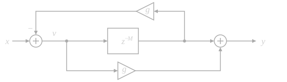
Solve the loop like before:
Then the output:
Take a look at the resulting equation. Notice anything? The numerator is an inversion of the denominator!
Proof 1: just multiply it out
On the circle \(z^{-M} = e^{-jM\theta}\). Call it \(w\) for short:
Numerator:
Denominator:
A total cancellation! Numerator over denominator is 1 at every frequency. The comb's 18 dB of ripple is defeated!
Proof 2: mirrors
Remember the unit circle figure from the EQ post? The gain is the distances to the zeros multiplied together, divided by the distances to the poles, times a fixed coefficient. So, we find them! Poles are where the denominator is zero, zeros are where the numerator is:
Identical angles. One radius is the mirror image of the other: \(r = g^{1/M}\) for the poles and \(1/r\) for the zeros. With our numbers that's 0.9978 and 1.0022, which means every zero is its pole.
"Standing" on the circle at \(e^{j\theta}\), with a pole at \(re^{j\beta}\) and its zero at \(\tfrac{1}{r}e^{j\beta}\), and pulling \(1/r\) out of the distance to the zero:
Law of cosines on what's left, and on the distance to the pole:
Identical lengths. So from anywhere on the circle, every zero is exactly \(1/r\) times as far away as its pole. Multiply all \(M\) pairs and zeros over poles is \((1/r)^M = 1/g\). The fixed number out front is \(g\) (write \(H = (gz^M + 1)/(z^M + g)\) and pull the \(g\) out of the top), so:
Every pole gets cancelled by its zero!
Proof 3: a 2×2 mirror
Linear algebra is great for diffusers and reverbs. Observe what happens in one sample. We've got the incoming signal, \(x\), and whatever the delay pipe outputs, call it \(d = v[n-M]\). Mixing those together using the equations above and we get the output, \(y\), plus a new \(v\) to send back into the pipe.
As a matrix:
Hmm.. still not pretty. Lets store a scaled version of \(v\) in the pipe: multiply it by \(c = \sqrt{1 - g^2}\). Call the scaled signals \(u = cv\) going in, and \(\tilde{d} = cd\) coming out, then put those into the two equations:
since \((1 - g^2)/c = c^2/c = c\). Now it's pretty:
\(g^2 + c^2 = 1\), so \(g\) and \(c\) are the cos and sin of some angle \(\alpha\):
A determinant of −1 means it's a mirror. The Diffusion knob literally tilts a mirror!
Multiply \(Q\) by its transpose (flipped over the diagonal):
The identity, so \(Q\) is orthogonal. Orthogonal matrices never change the length of a vector:
Which here means, every single sample:
Energy out the door plus energy into the pipe equals energy in the door plus energy out of the pipe. There's no leakage happening. Whatever goes in, comes out \(M\) samples later, over the whole signal \(\sum \tilde{d}^2 = \sum u^2\), and they cancel:
Energy out equals energy in, for any input at all. This is Parseval's theorem: the energy in time equals the energy across frequency:
If some frequency had a gain above 1, a sine there would come out with more energy than it went in, vice-versa. \(|H| = 1\) everywhere prevents this illegality. Chronos itself skips this rescale because it isn't necessary to achieve the desired allpass behaviour. This is an engineering decision: same allpass response at a fixed \(g\), without the extra scaling or having to manage differently scaled samples when \(g\) changes. Mostly rescaling is a maths trick to make the energy proof easier. It doesn't change the output.
Flat, but smeared
A flat response still does work! Consider the geometric series:
Multiply by \(r\):
Subtract, total cancellation with exception for the 1:
Backwards, \(1/(1 + gw)\) is a geometric series with \(r = -gw\). So the allpass expands to:
Lets group the terms by their power of \(w\). The constant term, \(w^0\), is just \(g\). For every higher power, \(w^n\), there are two ways to get there. Either multiply the \(w^n\) term in the series by \(g\), or multiply the \(w^{n-1}\) term by \(w\). Both give \(w^n\), so we add their coefficients:
\(w^n = z^{-nM}\) just means a delay of \(nM\) samples. So, hypothetically, if we fire off an impulse, we should get \(g\) out straight away, then the first echo \(M\) samples later. After that, another echo every \(M\) samples. Each one flips sign and is \(g\) multiplied by the size of the previous echo:
With our numbers: 0.78 at sample 0, then 0.392 at sample 113, −0.305 at 226, 0.238 at 339, so on, so forth.
Now, add up the energy (square every sample, sum them). Geometric series again, with \(r = g^2\):
Exactly 1! Unitary. A click with energy 1 goes in, energy 1 comes out, just spread over time.
How long does it ring? Every lap of the loop multiplies by \(g\). Falling 60 dB means a factor of 1000, so you need \(g^n = 1/1000\):
Turn \(g\) up and each echo keeps more of its level, and takes longer to fade out. On the diagram, that's the poles moving closer to the unit circle. Chronos caps \(g\) at 0.78.
The code
Snippet:
struct Allpass {
    std::vector<float> pipe;  // M samples long
    int w = 0;                 // where we are in the pipe
    float g = 0.0f;            // up to 0.78 in Chronos

    float process(float x) {
        float d = pipe[w];     // v[n - M]: went in M samples ago
        float v = x - g * d;   // the comb part
        pipe[w] = v;           // into the pipe
        w = (w + 1) % (int) pipe.size();
        return d + g * v;      // the part that flattens it
    }
};
Chronos essentially does the same arithmetic, with some cool software engineering optimizations.
How late is it?
This is the bit that actually matters for a delay plugin. If echoes are spread out, when does the repeat "arrive"? Check this:
The denominator is 1, and sample 0 adds nothing since \(n = 0\). The rest:
New series! Shift and subtract:
Plug it in:
Total \(g\) cancellation. Some of the sound comes out straight away, some comes out later. If you average those arrival times, and give louder bits more weight, you get exactly \(M\) samples. Turning Diffusion up smears more, but that average stays the same.
Phasing
We can get the same answer by looking at the phase, which also helps explain the smear. First, rewrite the numerator with \(w\) out front. On the unit circle, \(w\bar{w} = 1\), so \(g + w = w(1 + g\bar{w})\):
\(\overline{D}\) is \(D\)'s mirror image, same length and opposite angle. (Same length means flat. Proof 4.) So the phase is:
The first part, \(-M\theta\), is just a delay of \(M\) samples. The second part bends the phase back and forth. As \(w\) goes round the unit circle, \(D = 1 + gw\) traces a smaller circle centred at 1, with radius \(g\). Since \(g \lt 1\), that circle doesn't reach or wrap around zero. So \(D\)'s angle swings kind of like a pendulum, causing "bending", which produce smearing. Some frequencies get delayed less than \(M\) samples, others more. The delay at each frequency is minus the slope of the phase. Averaging it over a full lap cancel bits, leaving \(M\):
For an allpass, that average delay and the centre of mass are the same number (Parseval again, I'll spare you). The useful part is that phases add when you chain sections, so the delays add, so the centres of mass add.
Causality
Chronos's left channel adds up to 2923 samples at full Size, about 61 ms. Say the delay's on a quarter note at 120 bpm, so about 500 ms. Each lap now takes 561 ms on average, so a fourth repeat lands 244 ms late, too late and way off the grid!
So, how is this solved for? The centre of mass is exactly the sum of the lengths, so Chronos reads the delay line that much early:
439 ms of plain delay plus 61 ms of diffuser comes to 500 on the nose. Back in time!
Allpass Stacking
A single allpass keeps things tonally flat, but its echoes arrive late. That regular spacing still sounds buzzy. Run it through a few allpasses with different delay lengths and we get more echoes at different times. Their gains multiply, and each one has a gain of 1 at every frequency. So the whole chain stays flat:
Boom! Summation of delay taps. An echo that takes \(n_1\) laps through the first pipe and \(n_2\) through the second arrives after \(n_1M_1 + n_2M_2\) samples. How many have arrived by sample \(t\)? Lets say a grid just magically appears. Convenient huh? Let the x-axis of this grid = the first pipe's lap count across, and the y-axis be the second pipe's lap count up. Each dot is a single combination, and keeping the dots where \(n_1M_1 + n_2M_2 \le t\), these dots fill a triangle! Stretching occurs \(t/M_1\) across and \(t/M_2\) up, so we can roughly approximate the dots by taking the area:
With \(M_1 = 113\), \(M_2 = 167\) and \(t = 4800\) (100 ms) that's about 610. Accounting for dots on the edges, the real count is something like 648. One section on its own has 43. Extra sections add a power of \(t\), so \(K\) sections grow like the volume of a \(K\)-dimensional triangle:
This is including barely audible repeats. As stated before, taps degrade by \(g\) every lap. The earliest audible taps are actually quite early!
Prime Numbers Are Important
Our triangle assumes every dot is a different time, but that only works if the lengths don't share a factor. Try \(M_1 = 100\) and \(M_2 = 150\). Both are multiples of 50:
If both delays are multiples of 50, every echo has to hit on that same 50-sample grid. In the first 100 ms, we get 817 echoes sharing 96 arrival times. What does this mean? Too many echoes arriving in tandem creates an overlap instead of a spread. Some reinforce each other, others cancel. You get fewer separate arrivals, with a regular spacing that can sound metallic or buzzy rather than like a smooth wash. That regular spacing gives us a buzz at \(48000/50 = 960\) Hz. With 113 and 167, the 648 echoes in that same window all arrive at different samples.
So when do two different pairs clash?
If \(M_1\) and \(M_2\) share no factors, \(n_1 - n_1'\) has to be a multiple of \(M_2\). So the first clash can't come before:
100 and 150 clash after 300 samples, 6.25 ms. 113 and 167 go 18,871 samples, nearly 400 ms, way past where it even audibly matters.
Chronos's lengths
Chronos models a pretend room. Each channel gets about 21 metres of sound travel, split nine ways by a fixed ratio table. Metres to samples is just the speed of sound:
For the first section on the left, \(0.0396 \times 20.95 \approx 0.83\) m works out to 116.1 samples at 48 kHz, rounding down to 116. That would be cool if it weren't for the inconvenient fact that the number 116 isn't a prime. So, we use closest prime, 113 instead! Repeat for the other sections and we get 18 different prime lengths, 9 per side:
| Section | Left | Right |
|---|---|---|
| Plain 1 | 113 | 109 |
| Plain 2 | 167 | 163 |
| Plain 3 | 229 | 233 |
| Nested 1 (outer, inner) | 293, 181 | 307, 179 |
| Nested 2 | 431, 257 | 433, 263 |
| Nested 3 | 773, 479 | 787, 487 |
| Total | 2923 (60.9 ms) | 2961 (61.7 ms) |
Defining it in metres means it's the same room at any sample rate. The Size knob scales every length by the same factor, from 45% up to 100%, then performs a rounding:
So strictly speaking, they're only prime at full Size. The spread stays the same though.
Allpass Inception
Remember proof 1? It worked because \(w = z^{-M}\) has a magnitude of 1 at every frequency. That's all we needed from it. So we could swap that plain delay for something else with the same property. Another allpass, for example.
Lets try proof 1 again, replacing \(w\) with any \(B\) whose magnitude is 1. To multiply it out, use \(|a + b|^2 = |a|^2 + 2\operatorname{Re}(\bar{a}b) + |b|^2\). The bar at the top means we're dealing with a complex conjugate, and \(\operatorname{Re}\) means take the real part, as opposed to the imaginary. Since \(g\) is real, its conjugate is just \(g\):
Put \(|B| = 1\) in and both are \(1 + 2g\operatorname{Re}B + g^2\). Tonally Flat!
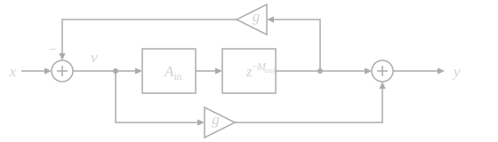
So instead of sending the signal straight into the pipe, send it through another allpass first:
On the circle \(|B| = |z^{-M_{\text{out}}}| \cdot |A_{\text{in}}| = 1 \cdot 1\), so \(H\) is an allpass. In matrix terms it's two mirrors and two pipes. The entire structure is energy-preserving.
Echo-wise it's a different beast. Every echo the inner allpass makes gets sent round the outer loop, and every lap of the outer loop goes back through the inner allpass. Echoes beget echoes. As for the delay itself, \(B\)'s phase winds down \(M_{\text{out}} + M_{\text{in}}\) times per lap of the circle, so the centre of mass is \(M_{\text{out}} + M_{\text{in}}\).
struct NestedAllpass {
    Allpass inner;             // a whole allpass in front of the pipe
    std::vector<float> pipe;  // the outer pipe
    int w = 0;
    float g = 0.0f;            // Chronos sets inner.g = 0.85f * g

    float process(float x) {
        float d = pipe[w];
        float v = x - g * d;
        pipe[w] = inner.process(v);   // through the inner allpass, then the pipe
        w = (w + 1) % (int) pipe.size();
        return d + g * v;
    }
};
Chronos runs three plain sections and then three nested ones, per channel.
Two ears
The LR channels use different primes (no length is shared) and slightly different rooms (20.95 m vs 21.075 m). Smearing happens on each channel differently, and that decorrelation creates width. Just how different exactly though? Treat each impulse response as one long vector and take the dot product:
Each one has unitary energy, so both lengths are 1 and \(\rho\) is just the dot product:
If \(\rho = 1\) is mono, 0 is max width. Different primes create echo variance between samples, so most of those products are zero and \(\rho\) ends up tiny
On the move
The human ear is amazing. Sometimes annoyingly so. SO MUCH SO that even after all this, at high diffusion, your brain will be able to pick out the subtle patterns in the trails! So naturally, we want some randomization, so the brain can't anticipate what's coming next.
A random walk on a leash
For this we use something called the Ornstein-Uhlenbeck (OU) process. Mean-reverting brownian motion. It's a leaky integrator. Every sample it keeps a fraction \(a\) of where it was and gets a random kick:
\(\xi\) is a fresh random number every sample (average 0, variance 1), and \(f_r\) is the Rate knob, which works like a cutoff. The \(a \cdot x\) part is what makes it mean-reverting while it gets shoved around.
Why \(\sqrt{1 - a^2}\)? When two signals are independent, their variances add up. Multiply a signal by \(a\) and its variance gets multiplied by \(a^2\). So once the variance settles at \(V\):
Exactly 1, regardless of rate. So you can see: Depth sets how far it wanders, and Rate sets how fast. The step is also exact. You get this formula by sampling a continuous OU process every \(1/f_s\) seconds, and you don't need to approximate!
A cheap bell curve
\(\xi\) is meant to be Gaussian, which just means random values that cluster around the middle in a bell-shaped curve (not unlike the bell curve meme). You can do something fraudulent and hack it by adding up four uniform random numbers, because each number is equally likely to land anywhere from 0 to 1:

Each \(u\) averages \(\tfrac{1}{2}\), with variance:
Adding all four here gives us an average of 2 and a variance of \(4/12 = 1/3\). Subtracting 2 centres it on 0, which we can then multiply by \(\sqrt{3}\) to bring the variance up to \(3 \cdot \tfrac{1}{3} = 1\). Adding enough independent random numbers gives us a bell curve result. This is what is called the central limit theorem. It could be more but 4 is enough, and it saves us some maths!
Doppler
Moving a delay tap bends the pitch. Read a sine through a delay \(d[n]\) that's changing:
Frequency is how fast the phase moves, so take the slope with respect to \(n\):
\(d'\) is how many samples the delay changes per sample. In cents (1200 to an octave), using \(\ln(1 + u) \approx u\) for small \(u\):
So pitch is the slope of the delay. Take a note of that. The tap also lands between samples now, so it has to interpolate, and interpolation is a whole world unto itself.
The slope problem
Here's the catch with OU. Look at how far it moves in one sample:
At slow rates \(a\) is super close to 1, so the first part is tiny, but the "kick" isn't. At 0.5 Hz:
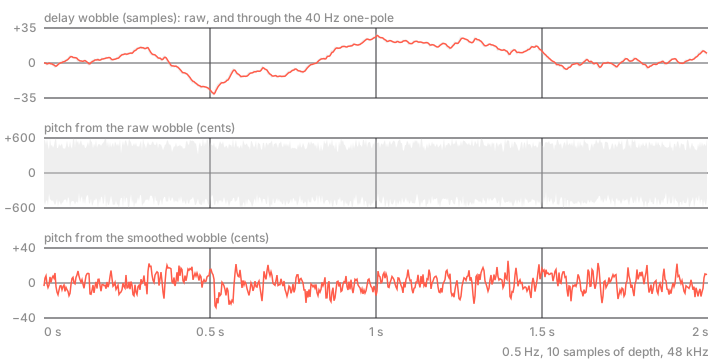
So each sample gets a random kick of about 0.0114. At about 10 samples of depth, that's roughly 0.11 samples of delay change per sample. This'll throw the pitch around by about 200-ish cents give-or-take, and with a fresh kick 48,000 times a second. All of this manifests as grit. This isn't good grit.
At smaller time steps this grit bcomes more intolerable. The kick scales like the square root of the time step interval, so the slope scales like its reciprocal:
OU, like Brownian motion, has no slope anywhere. Big problem after the Doppler bit.
These issues are fixed with a one-pole lowpass. Our new one-pole cuts down that gritty white noise above \(f_c = 40\) Hz. I'm going to break down what that looks like mathematically, and this'll make more sense if you work it out with me with pencil and paper, because I had to do that to really grasp it.
So. First, \(S_x(f)\) is the power spectral density of the OU wobble. It is what tells us how much variance lives around each frequency \(f\). We're using the continuous-time model here to get an estimate, counting both positive and negative frequencies. Its spectrum is:
\(\tau\) is the time constant, in seconds. Put its value into the top, then multiply the top and bottom by \(f_r^2\):
At this point, we need to take the derivative. That last equation tells us about the wobble \(x\). We want the spectrum of its slope \(x'\), where the prime (\(\prime\)) means a derivative with respect to time. We aren't differentiating that fraction with respect to \(f\), we're working out what taking the slope of the signal does to its power at each frequency. Simple calculus!
Starting with a single sine of amplitude \(A\), with \(t\) in seconds. The derivative of sine is cosine, and application of the chain rule means we also multiply by the derivative of \(2\pi f t\), which is \(2\pi f\):
Same frequency, but scaled \(2\pi f\) times the original. That's what I mean by "factor". Turning sine into cosine shifts the phase, and doesn't change the power. The differentiation is a geometric rotation across the unit circle. Multiplying the amplitude does change the power though, and since power depends on amplitude squared, the power gets multiplied by \((2\pi f)^2\).
The aforementioned rule applies to each frequency in the wobble too. The slope's power spectral density is the original power spectral density times \((2\pi f)^2\). Substitute \(S_x(f)\) with the fraction we just worked out:
Well above \(f_r\), \(f^2\) is much bigger than \(f_r^2\). I bet that looks like an assumption but ask yourself what "well above" means here: if \(f\) is 10 times \(f_r\), squaring makes \(f^2\) 100 times \(f_r^2\). This means we can drop the smaller term in the bottom:
The \(f^2\) cancels out, and thus reveals itself as the culprit: the slope sounds like white noise because we have equal power at every frequency! Without a lowpass, adding that flat spectrum up over all frequencies gives us infinite variance. We don't want that! Mean-reverting, remember?
The one-pole has this power response. The squared magnitude matters because we're filtering power:
Call the smoothed wobble \(x_s\). Filtering and taking a derivative can happen in either order, so multiply the slope's spectrum by that response:
The last line above uses the flat part of the raw slope's spectrum. It's a good estimate here because \(f_r = 0.5\) Hz is way below \(f_c = 40\) Hz. It slightly overestimates the power near zero.
The area under a power spectral density gives us the variance, written \(\sigma^2\). Pull the constant \(4\pi f_r\) outside the integral:
To do the integral, use \(u = f/f_c\). That means \(f = f_c u\) and \(df = f_c\,du\). Limits stay within infinity:
Sub that back in, then take the square root. At this point, you're probably thinking, "why \(\sqrt{1 - a^2}\)?". Well, independent things have variances that add, and scaling by \(a\) scales a variance by \(a^2\). So once it settles at some variance \(V\):
So that's the wobble's slope, per second. Multiplying by the depth nets us samples of delay change per second. Dividing by \(f_s\) gives us the change per sample:
Use the cents conversion from earlier to turn that into pitch wobble:
About 10 cents. 20 times calmer than the raw foolishness we were dealing with earlier. Hear it in action:
struct Wobble {
    double a = 1.0, s = 0.0, x = 0.0;  // leash, kick size, state (in sigmas)
    float k = 0.0f, lp = 0.0f;         // the 40 Hz one-pole

    void setRate(double rateHz, double fs) {
        a = std::exp(-2.0 * M_PI * rateHz / fs);
        s = std::sqrt(1.0 - a * a);                       // keeps the variance at 1
        k = 1.0f - (float) std::exp(-2.0 * M_PI * 40.0 / fs);
    }

    float next(Pcg32& rng) {
        float xi = (rng.nextUniform() + rng.nextUniform()
                  + rng.nextUniform() + rng.nextUniform() - 2.0f) * 1.7320508f;  // sqrt(3)
        x = std::clamp(a * x + s * xi, -4.0, 4.0);       // the OU step, on a 4 sigma leash
        lp += k * ((float) x - lp);                       // round the corners off
        return lp;                                        // times the depth, in samples
    }
};
What does it cost?
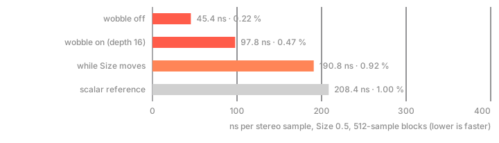
About 45 ns per stereo sample with the wobble off and 98 with it on (Chronos's diffuser_bench). At 48 kHz that's about 0.2% and 0.5% of one core.
Checking your work
Check the maths from this post directly:
- Flat. It multiplies out the exact \(H\) of all six sections at 8192 frequencies, and \(|H|\) has to be within 0.0001 of 1 at every one.
- Dense. It counts echoes above −60 dB in the first 100 ms (Size 0.5, \(g = 0.78\)), and there have to be more than the old design had, a plain chain of eight allpasses.
- No holes. The biggest gap between echoes in that first 100 ms has to be under 4 ms.
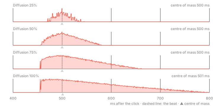
- On time. The centre of mass has to land within 1 sample of the summed lengths.
TL; DR
A delay with feedback is a comb, and a comb colours the sound. Add a feedforward tap and the top of \(H\) becomes the bottom written backwards. That's an allpass, flat at every frequency and smeared in time. The geometric series gives you the rest: its energy is exactly 1 and its centre of mass is exactly \(M\) samples, so Chronos reads the delay line early by the summed lengths and the repeats stay on the beat. Chain sections for density, use primes so the echoes don't stack up, nest them for more, and wobble them slowly with a random walk that's been through a one-pole.
References
This one leans on these. Any mistakes are mine.
- Manfred Schroeder and Ben Logan, "Colorless" Artificial Reverberation (1961): the allpass, and why combs colour.
- William G. Gardner, The Virtual Acoustic Room (MIT, 1992): nested allpasses.
- Jon Dattorro, Effect Design, Part 1: Reverberator and Other Filters (JAES, 1997): modulated allpass diffusers in a real reverb.
- Julius O. Smith III, Physical Audio Signal Processing (CCRMA): allpass filters, lossless systems and feedback delay networks.
- Jean-Marc Jot and Antoine Chaigne, Digital Delay Networks for Designing Artificial Reverberators (1991): feedback delay networks with orthogonal matrices.
- Geraint Luff (Signalsmith Audio), Let's Write a Reverb: Hadamard and Householder diffusion, super readable.