 Lissajous Labs
29 September 2026
So You Want to Make an EQ.. huh?
Nothing to it! A single EQ band is more or less, what? ~5 lines of arithmetic?
Disclaimer: The math here can seem kind of intimidating, especially if you're like me and try to visualize everything, but the concepts are more or less easy to digest. Spend some time with them; bonus points if you already know how to code.
What an EQ does
At its simplest it just makes targeted frequencies louder/quieter.
That's sort of... misleading though. Selectivity is actually quite a complex issue because of how sound is handled in the digital domain. You can't just arbitrarily turn stuff up/down, at least not without some VERY interesting mathematics, and clever use of \(\pi\):
Every frequency is a point on the unit circle, and so it sort of works like a frequency dial. At this point you may ask, why a circle? Most straightforward answer is that for something like digital frequencies (which wrap around), it's the easiest geometry on which to represent this process. DC is 0Hz, Nyquist (half whatever the sample rate is) is the highest frequency that can be represented within a given sample rate (for e.g, 24 kHz at 48 kHz). \(\textcolor{#79c0ff}{\cos\theta}, \textcolor{#ff5c4a}{\sin\theta}\) here are functioning as \(\textcolor{#79c0ff}{x}/\textcolor{#ff5c4a}{y}\) coordinates, and \(\textcolor{#e3b341}{\tan\theta}\) is where its extended radius crosses the line \(x = 1\); think of it as a sort of steepness function:
- 0°: the line is flat, so tan is 0.
- 45°: the line goes one up for one across, so tan is 1.
- 90°: the line points straight up, all climb and no across, so tan is infinite (∞).
- Past 90°: the line leans the other way, so tan goes negative.
It also should be said that tangent really starts to matter when we get into pre-warping, \(\textcolor{#e3b341}{g = \tan(\pi f/f_s)}\). The gain curve is interesting too: notice how it's drawn from the distances to the ○'s multiplied together, divided by the distances to the ×'s, times a fixed coefficient. Represented here is a bell: +12 dB at 8 kHz, Q of 1.5, at 48 kHz.
Make a note of these symbols:
| \(f_s\) | sample rate: samples per second, often 48,000 |
| \(T\) | time between samples, \(T = 1/f_s\) |
| \(f\) | a frequency in hertz |
| \(x, y\) | the filter's input and output, one number per sample |
| \(g\) | the tuning coefficient that sets the filter's frequency |
| \(Q\) | bandwidth: higher \(Q\) means a narrower band |
| \(k\) | \(1/Q\), which comes up often enough to get its own letter |
| \(s, z\) | the analog (continuous) and digital (sampled) domains |
Everything is a bucket
Simply put, almost every filter is constructed from a core component called an integrator (with some exceptions, like FIRs and direct-form biquads). The most appropriate mental model to adopt here is a bucket and water, where the water level at any moment is the total collected thus far. Literally like any bucket with water in it, under a pipe; the heavier the flow from the pipe, the faster the water level in the bucket rises etc etc, you get the idea. The water level isn't going to increase if the pipe is off. There's a "history" being "remembered"; That memory is the holding, the state held by the integrator. This is also just a capacitor.
Adding up a rate over time is integration. In DSP, the analog integrator is
or, with \(x\) as the water coming in and \(y\) as the water level,
\(1/s\) is just the level changed at the rate the water out of the pipe comes in!
Why is this important? Well, you get a filter by feeding some of an integrator's output back and subtracting it from its input. If you were to add it, the bucket would just overflow (sometimes dangerously).
Conversely, if you were to say, poke a hole in the bottom of the bucket so water leaks out at a rate proportional to how much water is held within, the water level would climb until water escapes as quickly as it is replaced, forming an equilibrium. At this point if you fiddle with the pipe and turn it up/down quickly, the less the water level will actually move because there isn't any time for it to catch up. Using this analogy I have described a Low-Pass filter, where the leak is the feedback, and the size of the leak is (more or less) your cutoff.
or, with \(\omega_c\) as the size of the leak,
Start stacking integrators in a loop and you can go from a one-pole smoother filter, to a trapezoidally integrated state-variable filter. And before you hit me with the "trap-a-you-say what-filter?", I want you to consider that computers can't integrate continuously!
Integrating with samples
As water from our metaphorical pipe flows (continuously), the water level is defined at every instant. A computer evaluates the signal 48,000 times per second, but it can't know about what's going on in between. So instead of integrating exactly, we need to estimate how much water arrived between two samples from the two readings we have.
Between sample \(n-1\) and sample \(n\) we know the flow rate at the start, \(x[n-1]\), and at the end, \(x[n]\). The simplest reasonable guess is that the rate change was linear. The water that arrived is then the area of a trapezoid: the width \(T\) times the average height.
Which is legit just the trapezoidal rule. Explained above, if you add new water to the previous level, you get a digital integrator:
Remember state, do some math, repeat. Easy peasy.
The bilinear transform
There is a lot of context packed in though. Writing \(z^{-1}\) for "one sample ago", so \(y[n-1]\) becomes \(z^{-1}Y\):
Collect the \(Y\) terms on the left and the \(X\) terms on the right:
The analog integrator was \(Y/X = 1/s\). These are the same integrator in two domains, so the domains must be related by
Which is the bilinear transform. Any analog filter written in terms of \(s\) can be moved into the digital domain with a simple substitution. The best part is that in our use-case it literally comes built-in. The trapezoidal rule and the bilinear transform are one and the same!
Frequency warping
Alright, lets continue with the metaphors. Picture a standard world map on a globe. If you were to try and superimpose this world map onto a rectangle, you'd fail. The usual projection stretches the regions near the poles, which is why Greenland looks about as big as Africa when Africa is fourteen times larger.
This folly is present in the bilinear transform. Where analog frequencies run from zero to infinity, digital frequencies stop at Nyquist. Immediately you can see the issue; trying to impose an infinite range into a finite one stretches the frequency axis, causing the warping to be at its worst offending toward the top.
In practice, a filter designed for some arbitrary frequency and sent through the transform as-is ends up acting at a lower frequency than intended. The solution here is to distort the request in the opposite direction first, so it's in the right place after the transform. This compensation step is called pre-warping, or \(g = \tan(\pi f/f_s)\).
To see how much the axis stretches, you should place a digital frequency \(\omega_d\) on the unit circle, \(z = e^{j\omega_d T}\), and send it through the substitution:
Things are going to get a bit hairy, but bear with me. The point sits at angle \(\omega_d T\) on the circle, so call half of that \(\phi = \omega_d T/2\):
Multiply the top and bottom by \(e^{j\phi}\). This is just multiplying by 1, so we end up with a matching pair (exponents add, so \(e^{j\phi} \cdot e^{-j2\phi} = e^{-j\phi}\)):
Here's where the unit circle comes back. \(e^{j\phi}\) is the point at angle \(\phi\), cos x-axis, and sin y-axis (\(j\) is a rotational vector of 90° counter-clockwise). \(e^{-j\phi}\) is its mirror image below the x-axis:
Subtract them and the cos parts cancel. Add them and the sin parts cancel:
Swap those into the top and bottom. The 2s cancel, and sin over cos is tan:
The \(j\)'s cancel, and putting \(\omega_d T/2\) back in for \(\phi\) leaves the exact relationship between the frequency you expect and the one you get:
So to make the digital filter act at frequency \(f\), tune it with
using \(\omega_c = 2\pi f\) and \(T = 1/f_s\).
Lets evaluate a simple example:
At \(f_s = 48{,}000\) and \(f = 1000\,\mathrm{Hz}\):
We'll keep reusing these numbers later. Plug them into the tan, and make sure your calculator's in radians, not degrees, or you'll get garbage:
So we have \(g \approx 0.0655\). Alright.
The one-pole filter and zero-delay feedback (ZDF)
Consider the humble one-pole lowpass. Construction is simple: one integrator with its output fed back to its input, and feedback is where things can get weird and people get stuck (historically, so did a fair number of textbooks).
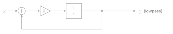
Let \(y\) be the integrator's output and \(s\) its stored state. The digital integrator's output is its state plus \(g\) multiplied by its input, where its input is the difference between the filter's input and output, \(x - y\).
\(y\) appears on both sides, so paradoxically, the output depends on itself in the same instant. This is an algebraic loop. So.. what do we do? The usual workaround is to just use the output from one sample ago, and while that does break the loop, it adds a delay the analog circuit doesn't have. This error compounds, and the filter's response suffers for it, predominantly at high cutoff frequencies.
Except you don't need a workaround. It's a linear equation, so solve it:
Exactly one value of \(y\) makes the loop consistent. No extra delay in the loop.
The code
Div every sample? NGMI bro. Fold \(1/(1 + g)\) into a coefficient that's computed once, whenever a knob turns:
Here it is in C++, with the state \(s\) renamed to z. It's the arithmetic of the one-pole in Chronos, line for line; Chronos adds a clamp on the frequency and computes the \(\tan\) with its own minimax approximation instead of std::tan. std trig functions are expensive and you can save a ton of cycles by using bounded approximations, but that's beyond scope here:
struct OnePoleTPT {
    double g = 0.0;  // tan(pi * fc / fs): the tuning coefficient
    double G = 0.0;  // g / (1 + g): the resolved coefficient
    double z = 0.0;  // the integrator's state

    void setCutoff(double fc, double fs) {
        g = std::tan(M_PI * fc / fs);
        G = g / (1.0 + g);            // once per knob move
    }

    double processLowpass(double x) {
        double v  = (x - z) * G;      // g * error: the delay-free part
        double lp = v + z;            // lowpass output
        z = lp + v;                   // trapezoidal state update
        return lp;                    // highpass = x - lp
    }
};
To check it matches the solution above, substitute \(G\) into \(\mathrm{lp} = v + z\): \(\bigl(g(x - z) + z(1 + g)\bigr) / (1 + g) = (gx + z) / (1 + g)\), and we achieve the same result! Our highpass comes free, too: \(x - \mathrm{lp}\).
With our numbers, \(G = 0.0655 / 1.0655 \approx 0.0615\). That's a working 1 kHz lowpass at 48 kHz.
The state-variable filter
You can only get a certain amount of spectrum tilt with a one-pole. It's a great parameter smoother, but for a heavy-duty equalizer we need more. We get our "more" with two integrators in a loop, or simply put, the state-variable filter.
The first signal in the loop is the highpass:
\(k = 1/Q\) sets how sharp the filter is. The first integrator turns the highpass into the bandpass, and the second turns the bandpass into the lowpass:
where \(s_1\) and \(s_2\) are the two integrators' states. As before, the unknowns appear on both sides.
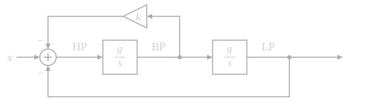
Solve for the bandpass first, since everything else follows. Substitute the definition of \(\mathrm{HP}\):
then substitute \(\mathrm{LP} = g \cdot \mathrm{BP} + s_2\), so that \(\mathrm{BP}\) is the only unknown:
Collect the \(\mathrm{BP}\) terms on the left:
The factor in parentheses is the determinant of the system. Naming the reciprocal, plus two products that keep turning up:
Then \(\mathrm{BP} = a_1 \cdot (gx + s_1 - g \cdot s_2)\), rearranges to the first line below. Feeding it into \(\mathrm{LP} = g \cdot \mathrm{BP} + s_2\) gives the second:
We get both outputs from the states, the input and three precomputed coefficients; isolating the term that refers to itself and dividing it out on a \(2 \times 2\) system.
State updates
Each integrator keeps a state for the next sample. The updates are short:
The \(2v - s\) form comes from the trapezoidal rule. An integrator's output is \(v = g \cdot u + s\), its state plus \(g\) multiplied by its input \(u\). The trapezoidal update for the next state is \(s \leftarrow v + g \cdot u\), and since \(g \cdot u = v - s\), that's \(v + (v - s) = 2v - s\). If you find yourself confused by all of this, fret not.
The Chronos implementation:
struct SVF {
    double g, k;                  // tan(pi * fc / fs) and 1/Q
    double a1, a2, a3;            // the solved loop coefficients
    double m0, m1, m2;            // output mix: the filter type (next section)
    double ic1 = 0.0, ic2 = 0.0;  // the two integrator states

    void setCoeff(double fc, double fs, double Q) {
        g  = std::tan(M_PI * fc / fs);
        k  = 1.0 / Q;
        a1 = 1.0 / (1.0 + g * (g + k));   // 1 / determinant
        a2 = g * a1;
        a3 = g * a2;
        // m0, m1, m2 depend on the filter type; see the next section
    }

    double step(double x) {
        double v3 = x - ic2;
        double v1 = a1 * ic1 + a2 * v3;         // BP
        double v2 = ic2 + a2 * ic1 + a3 * v3;   // LP
        ic1 = 2.0 * v1 - ic1;                   // trapezoidal
        ic2 = 2.0 * v2 - ic2;                   // state update
        return m0 * x + m1 * v1 + m2 * v2;      // mix
    }
};
Running the example through, with \(g \approx 0.0655\) and \(Q = 1/\sqrt{2}\) (so \(k = \sqrt{2} \approx 1.414\)):
And with that, we have a 1 kHz filter at 48 kHz!
Every filter type from one SVF
Each time the SVF runs, a bandpass and lowpass are computed, where the highpass is just \(x - k \cdot \mathrm{BP} - \mathrm{LP}\). So at every sample you have the signal split into low, band and high, and you can mix those back together in any proportion. That's what the step() function returns:
Three mix coefficients determine our filter behavior:
| Type | \(m_0\) | \(m_1\) | \(m_2\) | Effect |
|---|---|---|---|---|
| Lowpass | \(0\) | \(0\) | \(1\) | keeps the lows |
| Highpass | \(1\) | \(-k\) | \(-1\) | keeps the highs |
| Bandpass | \(0\) | \(k\) | \(0\) | keeps only the band around \(f\) |
| Notch | \(1\) | \(-k\) | \(0\) | removes only the band around \(f\) |
| Allpass | \(1\) | \(-2k\) | \(0\) | passes everything, shifts the phase |
Each row is a one-liner check. The highpass row gives \(x - k \cdot \mathrm{BP} - \mathrm{LP}\), which is how \(\mathrm{HP}\) was defined A Notch is the input minus the bandpass.
None of these is an EQ band yet. An EQ band boosts or cuts by a set amount, like +4 dB at 1 kHz, rather than passing or removing a band outright. Two more types, the bell and the shelf, are necessary. Those need decibels handled correctly.
Decibels, and why there's a 40
How much is +6 dB as a plain multiplier? Decibels are defined on power:
Power goes with the square of amplitude, so for an amplitude gain \(G_{\mathrm{amp}}\):
So +6 dB is roughly a factor of 2 in amplitude. Cool!
Not cool inside a bell or a shelf. The gain enters twice: it's applied along two paths through the two integrators, which multiply. So we parameterize these filters by the square root of the gain, called \(A\):
The 40 is the usual 20 with an extra factor of two, because \(A\) in this context is half the gain in decibels. This boost is correctly output as \(A^2\). Chronos computes \(A\) as \(\exp(\mathrm{gainDB} \cdot \ln 10 / 40)\), which is \(10^{\mathrm{dB}/40}\) written as an exponential to save CPU cycles.
It would be fair to expect +6 dB to become \(10^{6/20}\) everywhere, but a 20 would cause every boost and cut in the EQ to double in decibels: +6 dB comes out as +12.
Bells and shelves
With \(A\) defined, the EQ types are three more rows. The bell keeps the input flat and adds a scaled bandpass. The shelves scale the tuning coefficient by \(\sqrt{A}\), which keeps the transition centred on the desired frequency, and change the mix. The derivations are the same process as above (substitute, collect, solve) with quite a bit of bookkeeping; Andrew Simper's notes in the references have them in full. These are the values used in Chronos:
| Type | Tuning change | \(m_0\) | \(m_1\) | \(m_2\) |
|---|---|---|---|---|
| Bell | \(k \leftarrow k/A\) | \(1\) | \(k(A^2 - 1)\) | \(0\) |
| Low shelf | \(g \leftarrow g/\sqrt{A}\) | \(1\) | \(k(A - 1)\) | \(A^2 - 1\) |
| High shelf | \(g \leftarrow g \cdot \sqrt{A}\) | \(A^2\) | \(k \cdot A(1 - A)\) | \(1 - A^2\) |
That's an EQ band at the level of arithmetic. Pick a frequency (\(g\)), a \(Q\) (\(k\)) and a gain in decibels (\(A\)), fill in three mix coefficients, and run the loop.
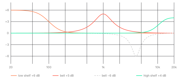
Each curve is one SVF with its own three mix coefficients. Chaining several = EQ.
From one band to an EQ
An EQ is a row of these bands in series. Signal passes through the first band, its output goes into the second, and so on. Low shelf? Bell? High shelf? Fundamentally these are just 3 copies of the same object.
What's left is mapping each band's knobs to its coefficients:
- frequency → \(g = \tan(\pi f / f_s)\)
- \(Q\) → \(k = 1/Q\)
- gain in dB → \(A = 10^{\mathrm{dB}/40}\), then the mix coefficients.
Details that matter in practice
Alright, now the.. less exciting (but still important!) stuff.
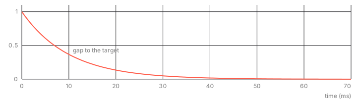
Smooth the coefficients. Normally if you turn a knob without parameter smoothing, you'll run up into something called Zipper Noise. Wholly unpleasant. This is solved in Chronos by setting new targets every 32 samples and nudging all six toward those targets every sample. This is legal: the SVF states are actual band signals (a direct-form biquad, not so much).
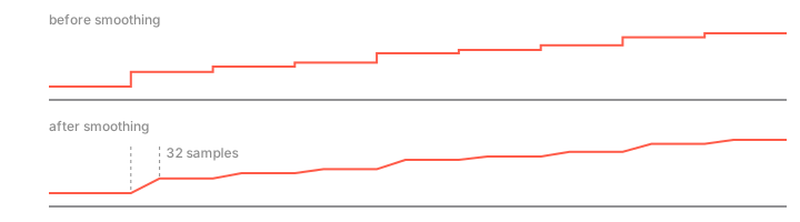
// once per 32-sample sub-block (setCoeffForBlock), shown for a1
const double a1_prior = a1;
setCoeff(type, sampleRate, freqHz, Q, gainDB);     // a1 now holds the target
da1 = (a1 - a1_prior) / numSamples;                // the per-sample step
a1 = a1_prior;                                     // start from where it was

// every sample (processBlockStep), after the filter step
a1 += da1;
Repeat for the other five!
Or, copy how a capacitor charges:
Guard against bad numbers. Feedback loops can make denormals. These are tiny numbers that'll slow a CPU down to a crawl. A NaN propagation or inf will kill the channel.
Draw the curve from the math. Don't run audio through the filter to draw the EQ curve. What you should do instead, is plug each pixel's frequency into the magnitude formula. This is what the magnitude() method is for!
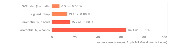
What does it cost? On an M1 Max all four bands come to 64 ns per stereo sample, about 0.3 % of one core.
Checking your work
Just because it runs doesn't mean it's correct! Two ways to check:
Kind of goes without saying, but measure first, cut once. If you fire an impulse through and FFT the output, you get the gain at every frequency. Compare it against the digital response, \(H(z)\) on the unit circle. Chronos has a check that runs 208 single-band settings plus a four-band cascade, bin by bin from 30 Hz to 20 kHz:
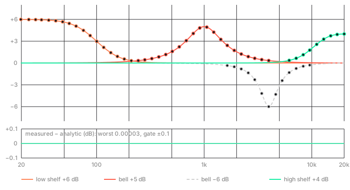
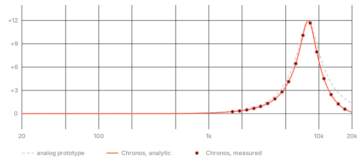
ParametricEQ. Lines are the math, rings are measured. The strip below is the difference, scaled to the ±0.1 dB limit.Do not however compare it to the analog prototype. It only lines up down low, because the bilinear transform crams everything up to infinity in below Nyquist. Here's the +12 dB, 8 kHz bell from the unit circle figure:
Second, just check the math by hand. All of this is maybe 2 pages of derivation.
TL; DR
A filter is integrators in a feedback loop. The trapezoidal rule (aka the bilinear transform) turns them into code. It squishes the frequency axis, so you prewarp with \(\tan\). The instantaneous feedback is just a linear equation you can solve. Two integrators make an SVF, and three mix coefficients make it any filter type, bells and shelves too (mind the 40). Put a few in series and you have an EQ.
References
This post stands on the shoulders of giants. These papers/books are critical reading; It's mostly the algebra they leave to the reader, written out. Any mistakes are mine.
- Vadim Zavalishin, The Art of VA Filter Design: the topology-preserving, zero-delay approach and the one-pole derivation.
- Andrew Simper (Cytomic), Solving the Continuous SVF Equations Using Trapezoidal Integration and Equivalent Currents and Linear Trapezoidal State Variable Filter: the SVF, its trapezoidal solution, the state update, and the bell and shelf mix coefficients.
- Robert Bristow-Johnson, Audio EQ Cookbook: the classic analog EQ prototypes and decibel conventions.
- Julius O. Smith III, online books at CCRMA: the bilinear transform and digital filters in general.